The following example constructs the Klein bottle as a simplicial complex K on 9 vertices, and then constructs the cellular chain complex C_∗=C_∗(K) from which the integral homology groups H_1(K, Z)= Z_2⊕ Z, H_2(K, Z)=0 are computed. The chain complex D_∗=C_∗ ⊗_ Z Z_2 is also constructed and used to compute the mod-2 homology vector spaces H_1(K, Z_2)= Z_2⊕ Z_2, H_2(K, Z)= Z_2. Finally, a presentation π_1(K) = ⟨ x,y : yxy^-1x⟩ is computed for the fundamental group of K.
gap> 2simplices:=
> [[1,2,5], [2,5,8], [2,3,8], [3,8,9], [1,3,9], [1,4,9],
>  [4,5,8], [4,6,8], [6,8,9], [6,7,9], [4,7,9], [4,5,7],
>  [1,4,6], [1,2,6], [2,6,7], [2,3,7], [3,5,7], [1,3,5]];;
gap> K:=SimplicialComplex(2simplices);
Simplicial complex of dimension 2.

gap> C:=ChainComplex(K);
Chain complex of length 2 in characteristic 0 .

gap> Homology(C,1);
[ 2, 0 ]
gap> Homology(C,2);
[  ]

gap> D:=TensorWithIntegersModP(C,2);
Chain complex of length 2 in characteristic 2 .

gap> Homology(D,1);
2
gap> Homology(D,2);
1

gap> G:=FundamentalGroup(K);
<fp group of size infinity on the generators [ f1, f2 ]>
gap> RelatorsOfFpGroup(G);
[ f2*f1*f2^-1*f1 ]
The following example constructs the real projective plane P, the Klein bottle K and the torus T as simplicial complexes, using the surface genus g as input in the oriented case and -g as input in the unoriented cases. It then confirms that the connected sums M=K#P and N=T#P have the same integral homology.
gap> P:=ClosedSurface(-1);
Simplicial complex of dimension 2.

gap> K:=ClosedSurface(-2);
Simplicial complex of dimension 2.

gap> T:=ClosedSurface(1);
Simplicial complex of dimension 2.

gap> M:=ConnectedSum(K,P);
Simplicial complex of dimension 2.

gap> N:=ConnectedSum(T,P);
Simplicial complex of dimension 2.

gap> Homology(M,0);
[ 0 ]
gap> Homology(N,0);
[ 0 ]
gap> Homology(M,1);
[ 2, 0, 0 ]
gap> Homology(N,1);
[ 2, 0, 0 ]
gap> Homology(M,2);
[  ]
gap> Homology(N,2);
[  ]
Given a group G one can consider the partially ordered set cal A_p(G) of all non-trivial elementary abelian p-subgroups of G, the partial order being set inclusion. The order complex ∆cal A_p(G) is a simplicial complex which is called the Quillen complex .
The following example constructs the Quillen complex ∆cal A_2(S_7) for the symmetric group of degree 7 and p=2. This simplicial complex involves 11291 simplices, of which 4410 are 2-simplices..
gap> K:=QuillenComplex(SymmetricGroup(7),2);
Simplicial complex of dimension 2.

gap> Size(K);
11291

gap> K!.nrSimplices(2);
4410
Any simplicial complex K can be regarded as a regular CW complex. Different datatypes are used in HAP for these two notions. The following continuation of the above Quillen complex example constructs a regular CW complex Y isomorphic to (i.e. with the same face lattice as) K=∆cal A_2(S_7). An advantage to working in the category of CW complexes is that it may be possible to find a CW complex X homotopy equivalent to Y but with fewer cells than Y. The cellular chain complex C_∗(X) of such a CW complex X is computed by the following commands. From the number of free generators of C_∗(X), which correspond to the cells of X, we see that there is a single 0-cell and 160 2-cells. Thus the Quillen complex $$\Delta{\cal A}_2(S_7) \simeq \bigvee_{1\le i\le 160} S^2$$ has the homotopy type of a wedge of 160 2-spheres. This homotopy equivalence is given in [Kso00, (15.1)] where it was obtained by purely theoretical methods.
gap> Y:=RegularCWComplex(K);
Regular CW-complex of dimension 2

gap> C:=ChainComplex(Y);
Chain complex of length 2 in characteristic 0 .

gap> C!.dimension(0);
1
gap> C!.dimension(1);
0
gap> C!.dimension(2);
160
For any regular CW complex Y one can look for a sequence of simple homotopy collapses Y↘ Y_1 ↘ Y_2 ↘ ... ↘ Y_N=X with X a smaller, and typically non-regular, CW complex. Such a sequence of collapses can be recorded using what is now known as a discrete vector field on Y. The sequence can, for example, be used to produce a chain homotopy equivalence f: C_∗ Y → C_∗ X and its chain homotopy inverse g: C_∗ X → C_∗ Y. The function ChainComplex(Y) returns the cellular chain complex C_∗(X), wheras the function ChainComplexOfRegularCWComplex(Y) returns the chain complex C_∗(Y).
For the above Quillen complex Y=∆cal A_2(S_7) the following commands produce the chain homotopy equivalence f: C_∗ Y → C_∗ X and g: C_∗ X → C_∗ Y. The number of generators of C_∗ Y equals the number of cells of Y in each degree, and this number is listed for each degree.
gap> K:=QuillenComplex(SymmetricGroup(7),2);;
gap> Y:=RegularCWComplex(K);;
gap> CY:=ChainComplexOfRegularCWComplex(Y);
Chain complex of length 2 in characteristic 0 .

gap> CX:=ChainComplex(Y);
Chain complex of length 2 in characteristic 0 .

gap> equiv:=ChainComplexEquivalenceOfRegularCWComplex(Y);;
gap> f:=equiv[1];
Chain Map between complexes of length 2 .

gap> g:=equiv[2];
Chain Map between complexes of length 2 .


gap> CY!.dimension(0);
1316
gap> CY!.dimension(1);
5565
gap> CY!.dimension(2);
4410
For some purposes one might need to simplify the cell structure on a regular CW-complex Y so as to obtained a homeomorphic CW-complex W with fewer cells.
The following commands load a 4-dimensional simplicial complex Y representing the K3 complex surface. Its simplicial structure is taken from [SK11] and involves 1704 cells of various dimensions. The commands then convert the cell structure into that of a homeomorphic regular CW-complex W involving 774 cells.
gap> Y:=RegularCWComplex(SimplicialK3Surface());
Regular CW-complex of dimension 4

gap> Size(Y);
1704
gap> W:=SimplifiedComplex(Y);
Regular CW-complex of dimension 4

gap> Size(W);
774
The following commands construct the complement M=S^3∖ K of the trefoil knot K. This complement is returned as a 3-manifold M with regular CW-structure involving four 3-cells.
gap> arc:=ArcPresentation(PureCubicalKnot(3,1));
[ [ 2, 5 ], [ 1, 3 ], [ 2, 4 ], [ 3, 5 ], [ 1, 4 ] ]
gap> S:=SphericalKnotComplement(arc);
Regular CW-complex of dimension 3

gap> S!.nrCells(3);
4
The following additional commands then show that M is homotopy equivalent to a reduced CW-complex Y of dimension 2 involving one 0-cell, two 1-cells and one 2-cell. The fundamental group of Y is computed and used to calculate the Alexander polynomial of the trefoil knot.
gap> Y:=ContractedComplex(S);
Regular CW-complex of dimension 2

gap> CriticalCells(Y);
[ [ 2, 1 ], [ 1, 9 ], [ 1, 11 ], [ 0, 22 ] ]
gap> G:=FundamentalGroup(Y);;
gap> AlexanderPolynomial(G);
x_1^2-x_1+1
The following example creates the projective plane Y as a regular CW-complex, and tests that it has the correct integral homology H_0(Y, Z)= Z, H_1(Y, Z)= Z_2, H_2(Y, Z)=0.
gap> attch:=RegularCWComplex_AttachCellDestructive;; #Function for attaching cells

gap> Y:=RegularCWDiscreteSpace(3); #Discrete CW-complex consisting of points {1,2,3}
Regular CW-complex of dimension 0

gap> e1:=attch(Y,1,[1,2]);; #Attach 1-cell
gap> e2:=attch(Y,1,[1,2]);; #Attach 1-cell
gap> e3:=attch(Y,1,[1,3]);; #Attach 1-cell
gap> e4:=attch(Y,1,[1,3]);; #Attach 1-cell
gap> e5:=attch(Y,1,[2,3]);; #Attach 1-cell
gap> e6:=attch(Y,1,[2,3]);; #Attach 1-cell
gap> f1:=attch(Y,2,[e1,e3,e5]);; #Attach 2-cell
gap> f2:=attch(Y,2,[e2,e4,e5]);; #Attach 2-cell
gap> f3:=attch(Y,2,[e2,e3,e6]);; #Attach 2-cell
gap> f4:=attch(Y,2,[e1,e4,e6]);; #Attach 2-cell
gap> Homology(Y,0);
[ 0 ]
gap> Homology(Y,1);
[ 2 ]
gap> Homology(Y,2);
[  ]`
The following example creates a 2-complex K corresponding to the group presentation
G=⟨ x,y,z : xyx^-1y^-1=1, yzy^-1z^-1=1, zxz^-1x^-1=1⟩.
The complex is shown to have the correct fundamental group and homology (since it is the 2-skeleton of the 3-torus S^1× S^1× S^1).
gap> S1:=RegularCWSphere(1);;
gap> W:=WedgeSum(S1,S1,S1);;
gap> F:=FundamentalGroupWithPathReps(W);; x:=F.1;;y:=F.2;;z:=F.3;;
gap> K:=RegularCWComplexWithAttachedRelatorCells(W,F,Comm(x,y),Comm(y,z),Comm(x,z));
Regular CW-complex of dimension 2

gap> G:=FundamentalGroup(K);
<fp group on the generators [ f1, f2, f3 ]>
gap> RelatorsOfFpGroup(G);
[ f2^-1*f1*f2*f1^-1, f1^-1*f3*f1*f3^-1, f2^-1*f3*f2*f3^-1 ]
gap> Homology(K,1);
[ 0, 0, 0 ]
gap> Homology(K,2);
[ 0, 0, 0 ]
The following example creats a 2-dimensional annulus A as a regular CW-complex, and testing that it has the correct integral homology H_0(A, Z)= Z, H_1(A, Z)= Z, H_2(A, Z)=0.
gap> FL:=[];; #The face lattice
gap> FL[1]:=[[1,0],[1,0],[1,0],[1,0]];;
gap> FL[2]:=[[2,1,2],[2,3,4],[2,1,4],[2,2,3],[2,1,4],[2,2,3]];;
gap> FL[3]:=[[4,1,2,3,4],[4,1,2,5,6]];;
gap> FL[4]:=[];;
gap> A:=RegularCWComplex(FL);
Regular CW-complex of dimension 2

gap> Homology(A,0);
[ 0 ]
gap> Homology(A,1);
[ 0 ]
gap> Homology(A,2);
[  ]
Next we construct the direct product Y=A× A× A× A× A of five copies of the annulus. This is a 10-dimensional CW complex involving 248832 cells. It will be homotopy equivalent Y≃ X to a CW complex X involving fewer cells. The CW complex X may be non-regular. We compute the cochain complex D_∗ = Hom_ Z(C_∗(X), Z) from which the cohomology groups
H^0(Y, Z)= Z,
H^1(Y, Z)= Z^5,
H^2(Y, Z)= Z^10,
H^3(Y, Z)= Z^10,
H^4(Y, Z)= Z^5,
H^5(Y, Z)= Z,
H^6(Y, Z)=0
are obtained.
gap> Y:=DirectProduct(A,A,A,A,A);
Regular CW-complex of dimension 10

gap> Size(Y);
248832
gap> C:=ChainComplex(Y);
Chain complex of length 10 in characteristic 0 .

gap> D:=HomToIntegers(C);
Cochain complex of length 10 in characteristic 0 .

gap> Cohomology(D,0);
[ 0 ]
gap> Cohomology(D,1);
[ 0, 0, 0, 0, 0 ]
gap> Cohomology(D,2);
[ 0, 0, 0, 0, 0, 0, 0, 0, 0, 0 ]
gap> Cohomology(D,3);
[ 0, 0, 0, 0, 0, 0, 0, 0, 0, 0 ]
gap> Cohomology(D,4);
[ 0, 0, 0, 0, 0 ]
gap> Cohomology(D,5);
[ 0 ]
gap> Cohomology(D,6);
[  ]
Strategy 1: Use geometric group theory in low dimensions.
Continuing with the previous example, we consider the first and fifth generators g_1^1, g_5^1∈ H^1(Y, Z) = Z^5 and establish that their cup product g_1^1 ∪ g_5^1 = - g_7^2 ∈ H^2(Y, Z) = Z^10 is equal to minus the seventh generator of H^2(Y, Z). We also verify that g_5^1∪ g_1^1 = - g_1^1 ∪ g_5^1.
gap> cup11:=CupProduct(FundamentalGroup(Y));
function( a, b ) ... end

gap> cup11([1,0,0,0,0],[0,0,0,0,1]);
[ 0, 0, 0, 0, 0, 0, -1, 0, 0, 0 ]

gap> cup11([0,0,0,0,1],[1,0,0,0,0]);
[ 0, 0, 0, 0, 0, 0, 1, 0, 0, 0 ]
This computation of low-dimensional cup products is achieved using group-theoretic methods to approximate the diagonal map ∆ : Y → Y× Y in dimensions ≤ 2. In order to construct cup products in higher degrees HAP invokes three further strategies.
Strategy 2: implement the Alexander-Whitney map for simplicial complexes.
For simplicial complexes the cup product is implemented using the standard formula for the Alexander-Whitney chain map, together with homotopy equivalences to improve efficiency.
As a first example, the following commands construct simplicial complexes K=( S^1 × S^1) # ( S^1 × S^1) and L=( S^1 × S^1) ∨ S^1 ∨ S^1 and establish that they have the same cohomology groups. It is then shown that the cup products ∪_K: H^2(K, Z)× H^2(K, Z) → H^4(K, Z) and ∪_L: H^2(L, Z)× H^2(L, Z) → H^4(L, Z) are antisymmetric bilinear forms of different ranks; hence K and L have different homotopy types.
gap> K:=ClosedSurface(2);
Simplicial complex of dimension 2.

gap> L:=WedgeSum(WedgeSum(ClosedSurface(1),Sphere(1)),Sphere(1));
Simplicial complex of dimension 2.

gap> Cohomology(K,0);Cohomology(L,0);
[ 0 ]
[ 0 ]
gap> Cohomology(K,1);Cohomology(L,1);
[ 0, 0, 0, 0 ]
[ 0, 0, 0, 0 ]
gap> Cohomology(K,2);Cohomology(L,2);
[ 0 ]
[ 0 ]
gap> gens:=[[1,0,0,0],[0,1,0,0],[0,0,1,0],[0,0,0,1]];;
gap> cupK:=CupProduct(K);;
gap> cupL:=CupProduct(L);;
gap> A:=NullMat(4,4);;B:=NullMat(4,4);;
gap> for i in [1..4] do
> for j in [1..4] do
> A[i][j]:=cupK(1,1,gens[i],gens[j])[1];
> B[i][j]:=cupL(1,1,gens[i],gens[j])[1];
> od;od;
gap> Display(A);
[ [   0,   0,   0,   1 ],
  [   0,   0,   1,   0 ],
  [   0,  -1,   0,   0 ],
  [  -1,   0,   0,   0 ] ]
gap> Display(B);
[ [   0,   1,   0,   0 ],
  [  -1,   0,   0,   0 ],
  [   0,   0,   0,   0 ],
  [   0,   0,   0,   0 ] ]
gap> Rank(A);
4
gap> Rank(B);
2
As a second example of the computation of cups products, the following commands construct the connected sums V=M# M and W=M# overline M where M is the K3 complex surface which is stored as a pure simplicial complex of dimension 4 and where overline M denotes the opposite orientation on M. The simplicial structure on the K3 surface is taken from [SK11]. The commands then show that H^2(V, Z)=H^2(W, Z)= Z^44 and H^4(V, Z)=H^4(W, Z)= Z. The final commands compute the matrix AV=(x∪ y) as x,y range over a generating set for H^2(V, Z) and the corresponding matrix AW for W. These two matrices are seen to have a different number of positive eigenvalues from which we can conclude that V is not homotopy equivalent to W.
gap> M:=SimplicialK3Surface();;
gap> V:=ConnectedSum(M,M,+1);
Simplicial complex of dimension 4.

gap> W:=ConnectedSum(M,M,-1);
Simplicial complex of dimension 4.

gap> Cohomology(V,2);
[ 0, 0, 0, 0, 0, 0, 0, 0, 0, 0, 0, 0, 0, 0, 0, 0, 0, 0, 0, 0, 0, 0, 0, 0, 0,
  0, 0, 0, 0, 0, 0, 0, 0, 0, 0, 0, 0, 0, 0, 0, 0, 0, 0, 0 ]
gap> Cohomology(W,2);
[ 0, 0, 0, 0, 0, 0, 0, 0, 0, 0, 0, 0, 0, 0, 0, 0, 0, 0, 0, 0, 0, 0, 0, 0, 0,
  0, 0, 0, 0, 0, 0, 0, 0, 0, 0, 0, 0, 0, 0, 0, 0, 0, 0, 0 ]
gap> Cohomology(V,4);
[ 0 ]
gap> Cohomology(W,4);
[ 0 ]
gap> cupV:=CupProduct(V);;
gap> cupW:=CupProduct(W);;
gap> AV:=NullMat(44,44);;
gap> AW:=NullMat(44,44);;
gap> gens:=IdentityMat(44);;
gap> for i in [1..44] do
> for j in [1..44] do
> AV[i][j]:=cupV(2,2,gens[i],gens[j])[1];
> AW[i][j]:=cupW(2,2,gens[i],gens[j])[1];
> od;od;
gap> SignatureOfSymmetricMatrix(AV);
rec( determinant := 1, negative_eigenvalues := 22, positive_eigenvalues := 22,
  zero_eigenvalues := 0 )
gap> SignatureOfSymmetricMatrix(AW);
rec( determinant := 1, negative_eigenvalues := 6, positive_eigenvalues := 38,
  zero_eigenvalues := 0 )
A cubical cubical version of the Alexander-Whitney formula, due to J.-P. Serre, could be used for computing the cohomology ring of a regular CW-complex whose cells all have a cubical combinatorial face lattice. This has not been implemented in HAP. However, the following more general approach has been implemented.
Strategy 3: Implement a cellular approximation to the diagonal map on an arbitrary finite regular CW-complex.
The following example calculates the cup product H^2(W, Z)× H^2(W, Z) → H^4(W, Z) for the 4-dimensional orientable manifold W=M× M where M is the closed surface of genus 2. The manifold W is stored as a regular CW-complex.
gap> M:=RegularCWComplex(ClosedSurface(2));;
gap> W:=DirectProduct(M,M);
Regular CW-complex of dimension 4

gap> Size(W);
5776
gap> W:=SimplifiedComplex(W);;
gap> Size(W);
1024

gap> Homology(W,2);
[ 0, 0, 0, 0, 0, 0, 0, 0, 0, 0, 0, 0, 0, 0, 0, 0, 0, 0 ]
gap> Homology(W,4);
[ 0 ]

gap> cup:=CupProduct(W);;
gap> SecondCohomologtGens:=IdentityMat(18);;
gap> A:=NullMat(18,18);;
gap> for i in [1..18] do
> for j in [1..18] do
> A[i][j]:=cup(2,2,SecondCohomologtGens[i],SecondCohomologtGens[j])[1];
> od;od;
gap> Display(A);
[ [    0,   -1,    0,    0,    0,    0,    3,   -2,    0,    0,    0,    1,   -1,    0,    0,    1,    0,    0 ],
  [   -1,  -10,    1,    2,   -2,    1,    6,   -1,    0,   -3,    4,   -1,   -1,   -1,    4,   -2,   -2,    0 ],
  [    0,    1,   -2,    1,    0,   -1,    0,    0,    1,    0,   -1,    1,    0,    0,    1,   -1,    0,    0 ],
  [    0,    2,    1,   -2,    1,    0,    0,   -1,    0,    1,    0,    0,    0,    0,   -1,    2,    0,    0 ],
  [    0,   -2,    0,    1,    0,    0,    1,   -1,    0,    0,   -1,    0,    0,    0,    0,   -1,    0,    0 ],
  [    0,    1,   -1,    0,    0,    0,    0,    1,   -1,    1,    0,    0,    0,    0,    1,   -1,    0,    0 ],
  [    3,    6,    0,    0,    1,    0,   -4,    0,   -1,    2,    4,   -5,    2,   -1,    1,    0,    3,    0 ],
  [   -2,   -1,    0,   -1,   -1,    1,    0,    4,   -2,    0,    0,    3,   -1,    1,   -1,    0,   -2,    0 ],
  [    0,    0,    1,    0,    0,   -1,   -1,   -2,    4,   -3,  -10,    1,    0,    0,   -3,    3,    0,    0 ],
  [    0,   -3,    0,    1,    0,    1,    2,    0,   -3,    2,    3,    0,    0,    0,    1,   -3,    0,    0 ],
  [    0,    4,   -1,    0,   -1,    0,    4,    0,  -10,    3,   18,    1,    0,    0,    0,    4,    0,    1 ],
  [    1,   -1,    1,    0,    0,    0,   -5,    3,    1,    0,    1,    0,    0,    0,   -2,   -1,   -1,    0 ],
  [   -1,   -1,    0,    0,    0,    0,    2,   -1,    0,    0,    0,    0,    0,    0,    1,    0,    0,    0 ],
  [    0,   -1,    0,    0,    0,    0,   -1,    1,    0,    0,    0,    0,    0,    0,    0,   -1,   -1,    0 ],
  [    0,    4,    1,   -1,    0,    1,    1,   -1,   -3,    1,    0,   -2,    1,    0,    0,    2,    2,    0 ],
  [    1,   -2,   -1,    2,   -1,   -1,    0,    0,    3,   -3,    4,   -1,    0,   -1,    2,    0,    0,    0 ],
  [    0,   -2,    0,    0,    0,    0,    3,   -2,    0,    0,    0,   -1,    0,   -1,    2,    0,    0,    0 ],
  [    0,    0,    0,    0,    0,    0,    0,    0,    0,    0,    1,    0,    0,    0,    0,    0,    0,    0 ] ]

gap> SignatureOfSymmetricMatrix(A);
rec( determinant := -1, negative_eigenvalues := 9, positive_eigenvalues := 9,
  zero_eigenvalues := 0 )
The matrix A representing the cup product H^2(W, Z)× H^2(W, Z) → H^4(W, Z) is shown to have 9 positive eigenvalues, 9 negative eigenvalues, and no zero eigenvalue.
Strategy 4: Guess and verify a cellular approximation to the diagonal map.
Many naturally occuring cell structures are neither simplicial nor cubical. For a general regular CW-complex we can attempt to construct a cellular inclusion overline Y ↪ Y× Y with {(y,y) : y∈ Y}⊂ overline Y and with projection p: overline Y ↠ Y that induces isomorphisms on integral homology. The function DiagonalApproximation(Y) constructs a candidate inclusion, but the projection p: overline Y ↠ Y needs to be tested for homology equivalence. If the candidate inclusion passes this test then the function CupProductOfRegularCWComplex_alt(Y), involving the candidate space, can be used for cup products. (I think the test is passed for all regular CW-complexes that are subcomplexes of some Euclidean space with all cells convex polytopes -- but a proof needs to be written down!)
The following example calculates g_1^2 ∪ g_2^2 ne 0 where Y=T× T is the direct product of two copies of a simplicial torus T, and where g_k^n denotes the k-th generator in some basis of H^n(Y, Z). The direct product Y is a CW-complex which is not a simplicial complex.
gap> K:=RegularCWComplex(ClosedSurface(1));;
gap> Y:=DirectProduct(K,K);;
gap> cup:=CupProductOfRegularCWComplex_alt(Y);;
gap> cup(2,2,[1,0,0,0,0,0],[0,1,0,0,0,0]);
[ 5 ]

gap> D:=DiagonalApproximation(Y);;
gap> p:=D!.projection;
Map of regular CW-complexes

gap> P:=ChainMap(p);
Chain Map between complexes of length 4 .

gap> IsIsomorphismOfAbelianFpGroups(Homology(P,0));
true
gap> IsIsomorphismOfAbelianFpGroups(Homology(P,2));
true
gap> IsIsomorphismOfAbelianFpGroups(Homology(P,3));
true
gap> IsIsomorphismOfAbelianFpGroups(Homology(P,4));
true
Of course, either of Strategies 2 or 3 could also be used for this example. To use the Alexander-Whitney formula of Strategy 2 we would need to give the direct product Y=T× T a simplicial structure. This could be obtained using the function DirectProduct(T,T). The details are as follows. (The result is consistent with the preceding computation since the choice of a basis for cohomology groups is far from unique.)
gap> K:=ClosedSurface(1);;
gap> KK:=DirectProduct(K,K);
Simplicial complex of dimension 4.

gap> cup:=CupProduct(KK);;
gap> cup(2,2,[1,0,0,0,0,0],[0,1,0,0,0,0]);
[ 0 ]
The cup product gives rise to the intersection form of a connected, closed, orientable 4-manifold Y is a symmetric bilinear form
qY: H^2(Y, Z)/Torsion × H^2(Y, Z)/Torsion ⟶ Z
which we represent as a symmetric matrix.
The following example constructs the direct product L=S^2× S^2 of two 2-spheres, the connected sum M= CP^2 # overline CP^2 of the complex projective plane CP^2 and its oppositely oriented version overline CP^2, and the connected sum N= CP^2 # CP^2. The manifolds L, M and N are each shown to have a CW-structure involving one 0-cell, two 1-cells and one 2-cell. They are thus simply connected and have identical cohomology.
gap> S:=Sphere(2);;
gap> S:=RegularCWComplex(S);;
gap> L:=DirectProduct(S,S);
Regular CW-complex of dimension 4

gap> M:=ConnectedSum(ComplexProjectiveSpace(2),ComplexProjectiveSpace(2),-1);
Simplicial complex of dimension 4.

gap> N:=ConnectedSum(ComplexProjectiveSpace(2),ComplexProjectiveSpace(2),+1);
Simplicial complex of dimension 4.

gap> CriticalCells(L);
[ [ 4, 1 ], [ 2, 13 ], [ 2, 56 ], [ 0, 16 ] ]
gap> CriticalCells(RegularCWComplex(M));
[ [ 4, 1 ], [ 2, 109 ], [ 2, 119 ], [ 0, 8 ] ]
gap> CriticalCells(RegularCWComplex(N));
[ [ 4, 1 ], [ 2, 119 ], [ 2, 149 ], [ 0, 12 ] ]
John Milnor showed (as a corollary to a theorem of J. H. C. Whitehead) that the homotopy type of a simply connected 4-manifold is determined by its quadratic form. More precisely, a form is said to be of type I (properly primitive) if some diagonal entry of its matrix is odd. If every diagonal entry is even, then the form is of type II (improperly primitive). The index of a form is defined as the number of positive diagonal entries minus the number of negative ones, after the matrix has been diagonalized over the real numbers.
Theorem. (Milnor [Mil58]) The oriented homotopy type of a simply connected, closed, orientable 4-manifold is determined by its second Betti number and the index and type of its intersetion form; except possibly in the case of a manifold with definite quadratic form of rank r > 9.
The following commands compute matrices representing the intersection forms qL, qM, qN.
gap> qL:=IntersectionForm(L);;
gap> qM:=IntersectionForm(M);;
gap> qN:=IntersectionForm(N);;
gap> Display(qL);
[ [  -2,   1 ],
  [   1,   0 ] ]
gap> Display(qM);
[ [  1,  0 ],
  [  0,  1 ] ]
gap> Display(qN);
[ [   1,   0 ],
  [   0,  -1 ] ]
Since qL is of type II, whereas qM and qN are of type I we see that the oriented homotopy type of L is distinct to that of M and that of N. Since qM has index 2 and qN has index 0 we see that that M and N also have distinct oriented homotopy types.
The cup product gives the cohomology H^∗(X,R) of a space X with coefficients in a ring R the structure of a graded commutitive ring. The function CohomologyRing(Y,p) returns the cohomology as an algebra for Y a simplicial complex and R= Z_p the field of p elements. For more general regular CW-complexes or R= Z the cohomology ring structure can be determined using the function CupProduct(Y).
The folowing commands compute the mod 2 cohomology ring H^∗(W, Z_2) of the above wedge sum W=M∨ N of a 2-dimensional orientable simplicial surface of genus 2 and the K3 complex simplicial surface (of real dimension 4).
gap> M:=ClosedSurface(2);;
gap> N:=SimplicialK3Surface();;
gap> W:=WedgeSum(M,N);;
gap> A:=CohomologyRing(W,2);
<algebra of dimension 29 over GF(2)>
gap> x:=Basis(A)[25];
v.25
gap> y:=Basis(A)[27];
v.27
gap> x*y;
v.29
The functions CupProduct and IntersectionForm can be used to determine integral cohomology rings. For example, the integral cohomology ring of an arbitrary closed surface was calculated in [GM15, Theorem 3.5]. For any given surface M this result can be recalculated using the intersection form. For instance, for an orientable surface of genus g it is well-known that H^1(M, Z)= Z^2g, H^2(M, Z)= Z. The ring structure multiplication is thus given by the matrix of the intersection form. For say g=3 the ring multiplication is given, with respect to some cohomology basis, in the following.
gap> M:=ClosedSurface(3);;
gap> Display(IntersectionForm(M));
[ [   0,   0,   1,  -1,  -1,   0 ],
  [   0,   0,   0,   1,   1,   0 ],
  [  -1,   0,   0,   1,   1,  -1 ],
  [   1,  -1,  -1,   0,   0,   1 ],
  [   1,  -1,  -1,   0,   0,   0 ],
  [   0,   0,   1,  -1,   0,   0 ] ]
By changing the basis B for H^1(M, Z) we obtain the following simpler matrix representing multiplication in H^∗(M, Z).
gap> B:=[ [ 0, 1, -1, -1, 1, 0 ],
>         [ 1, 0, 1, 1, 0, 0 ],
>         [ 0, 0, 1, 0, 0, 0 ],
>         [ 0, 0, 0, 1, -1, 0 ],
>         [ 0, 0, 1, 1, 0, 0 ],
>         [ 0, 0, 1, 1, 0, 1 ] ];;
gap> Display(IntersectionForm(M,B));
[ [   0,   1,   0,   0,   0,   0 ],
  [  -1,   0,   0,   0,   0,   0 ],
  [   0,   0,   0,   0,   1,   0 ],
  [   0,   0,   0,   0,   0,   1 ],
  [   0,   0,  -1,   0,   0,   0 ],
  [   0,   0,   0,  -1,   0,   0 ] ]
The following example evaluates the Bockstein homomorphism β_2: H^∗(X, Z_2) → H^∗ +1(X, Z_2) on an additive basis for X=Σ^100( RP^2 × RP^2) the 100-fold suspension of the direct product of two projective planes.
gap> P:=SimplifiedComplex(RegularCWComplex(ClosedSurface(-1)));
Regular CW-complex of dimension 2
gap> PP:=DirectProduct(P,P);;
gap> SPP:=Suspension(PP,100);
Regular CW-complex of dimension 104
gap> A:=CohomologyRing(SPP,2);
<algebra of dimension 9 over GF(2)>
gap> List(Basis(A),x->Bockstein(A,x));
[ 0*v.1, v.4, v.6, 0*v.1, v.7+v.8, 0*v.1, v.9, v.9, 0*v.1 ]
If only the Bockstein homomorphism is required, and not the cohomology ring structure, then the Bockstein could also be computedirectly from a chain complex. The following computes the Bockstein β_2: H^2(Y, Z_2) → H^3(Y, Z_2) for the direct product Y=K × K × K × K of four copies of the Klein bottle represented as a regular CW-complex with 331776 cells. The order of the kernel and image of β_2 are computed.
gap> K:=ClosedSurface(-2);;
gap> K:=SimplifiedComplex(RegularCWComplex(K));;
gap> KKKK:=DirectProduct(K,K,K,K);
Regular CW-complex of dimension 8
gap> Size(KKKK);
331776
gap> C:=ChainComplex(KKKK);;
gap> bk:=Bockstein(C,2,2);;
gap> Order(Kernel(bk));
1024
gap> Order(Image(bk));
262144
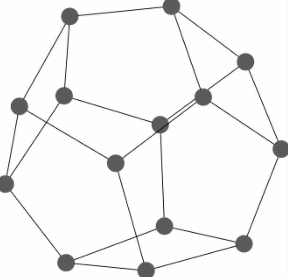
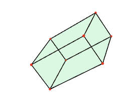
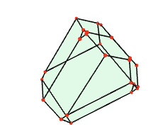
By a diagonal approximation on a regular CW-complex X we mean any cellular map ∆: X→ X× X that is homotopic to the diagonal map X→ X× X, x↦ (x,x) and equal to the diagonal map when restricted to the 0-skeleton. Theoretical formulae for diagonal maps on a polytope X can have interesting combinatorial aspects. To illustrate this let us consider, for n=3, the n-dimensional polytope cal K^n+2 known as the associahedron. The following commands display the 1-skeleton of cal K^5.
gap> n:=3;;Y:=RegularCWAssociahedron(n+2);;
gap> Display(GraphOfRegularCWComplex(Y));
The induced chain map C_∗(cal K^n+2) → C_∗(cal K^n+2× cal K^n+2) sends the unique free generator e^n_1 of C_n(cal K^n+2) to a sum ∆(e^n_1) of a number of distinct free generators of C_n(cal K^n+2× cal K^n+2). Let |∆(e^n_1)| denote the number of free generators. For n=3 the following commands show that |∆(e^3_1)|=22 with each free generator occurring with coefficient ± 1.
gap> n:=3;;Y:=RegularCWAssociahedron(n+2);;
gap> D:=DiagonalChainMap(Y);;Filtered(D!.mapping([1],n),x->x<>0);
[ 1, 1, -1, -1, 1, 1, -1, -1, 1, -1, 1, 1, -1, 1, 1, 1, -1, -1, 1, 1, 1, 1 ]
Repeating this example for 0≤ n≤ 6 yields the sequence |∆(e^n_1)|: 1, 2, 6, 22, 91, 408, 1938, ⋯. The On-line Encyclopedia of Integer Sequences explains that this is the beginning of the sequence given by the number of canopy intervals in the Tamari lattices.
Repeating the same experiment for the permutahedron, using the command RegularCWPermutahedron(n), yields the sequence |∆(e^n_1)|: 1, 2, 8, 50, 432, 4802,⋯. The On-line Encyclopedia of Integer Sequences explains that this is the beginning of the sequence given by the number of spanning trees in the graph K_n/e, which results from contracting an edge e in the complete graph K_n on n vertices.
Repeating the experiment for the cube, using the command RegularCWCube(n), yields the sequence |∆(e^n_1)|: 1, 2, 4, 8, 16, 32,⋯.
Repeating the experiment for the simplex, using the command RegularCWSimplex(n), yields the sequence |∆(e^n_1)|: 1, 2, 3, 4, 5, 6,⋯.
A strictly cellular map f: X→ Y of regular CW-complexes is a cellular map for which the image of any cell is a cell (of possibly lower dimension). Inclusions of CW-subcomplexes, and projections from a direct product to a factor, are examples of such maps. Strictly cellular maps can be represented in HAP, and their induced homomorphisms on (co)homology and on fundamental groups can be computed.
The following example begins by visualizing the trefoil knot κ ∈ R^3. It then constructs a regular CW structure on the complement Y= D^3∖ Nbhd(κ) of a small tubular open neighbourhood of the knot lying inside a large closed ball D^3. The boundary of this tubular neighbourhood is a 2-dimensional CW-complex B homeomorphic to a torus S^1× S^1 with fundamental group π_1(B)=<a,b : aba^-1b^-1=1>. The inclusion map f: B↪ Y is constructed. Then a presentation π_1(Y)= <x,y | xy^-1x^-1yx^-1y^-1> and the induced homomorphism $$\pi_1(B)\rightarrow \pi_1(Y), a\mapsto y^{-1}xy^2xy^{-1}, b\mapsto y $$ are computed. This induced homomorphism is an example of a peripheral system and is known to contain sufficient information to characterize the knot up to ambient isotopy.
Finally, it is verified that the induced homology homomorphism H_2(B, Z) → H_2(Y, Z) is an isomomorphism.
gap> K:=PureCubicalKnot(3,1);;
gap> ViewPureCubicalKnot(K);;

gap> K:=PureCubicalKnot(3,1);;
gap> f:=KnotComplementWithBoundary(ArcPresentation(K));
Map of regular CW-complexes

gap> G:=FundamentalGroup(Target(f));
<fp group of size infinity on the generators [ f1, f2 ]>
gap> RelatorsOfFpGroup(G);
[ f1*f2^-1*f1^-1*f2*f1^-1*f2^-1 ]

gap> F:=FundamentalGroup(f);
[ f1, f2 ] -> [ f2^-1*f1*f2^2*f1*f2^-1, f1 ]


gap> phi:=ChainMap(f);
Chain Map between complexes of length 2 .

gap> H:=Homology(phi,2);
[ g1 ] -> [ g1 ]
The following example constructs a 3-dimensional pure regular CW-complex K whose 3-cells are permutahedra. It then constructs the simplicial complex B by taking barycentric subdivision. It then constructes a smaller, homotopy equivalent, simplicial complex N by taking the nerve of the cover of K by the closures of its 3-cells.
gap> K:=RegularCWComplex(PureComplexComplement(PurePermutahedralKnot(3,1)));
Regular CW-complex of dimension 3

gap> Size(K);
77923
gap> B:=BarycentricSubdivision(K);
Simplicial complex of dimension 3.

gap> Size(B);
1622517
gap> N:=Nerve(K);
Simplicial complex of dimension 3.

gap> Size(N);
48745
By a classifying space for a group G we mean a path-connected space BG with fundamental group π_1(BG)≅ G isomorphic to G and with higher homotopy groups π_n(BG)=0 trivial for all n≥ 2. The homology of the group G can be defined to be the homology of BG: H_n(G, Z) = H_n(BG, Z).
In principle BG can always be constructed as a regular CW-complex. For instance, the following extremely slow commands construct the 5-skeleton Y^5 of a regular CW-classifying space Y=BG for the dihedral group of order 16 and use it to calculate H_1(G, Z)= Z_2⊕ Z_2, H_2(G, Z)= Z_2, H_3(G, Z)= Z_2⊕ Z_2 ⊕ Z_8, H_4(G, Z)= Z_2 ⊕ Z_2. The final command shows that the constructed space Y^5 in this example is a 5-dimensional regular CW-complex with a total of 15289 cells.
gap> Y:=ClassifyingSpaceFiniteGroup(DihedralGroup(16),5);
Regular CW-complex of dimension 5
gap> Homology(Y,1);
[ 2, 2 ]
gap> Homology(Y,2);
[ 2 ]
gap> Homology(Y,3);
[ 2, 2, 8 ]
gap> Homology(Y,4);
[ 2, 2 ]
gap> Size(Y);
15289
The n-skeleton of a regular CW-classifying space of a finite group necessarily involves a large number of cells. For the group G=C_2 of order two a classifying space can be take to be real projective space BG= RP^∞ with n-skeleton BG^n= RP^n. To realize BG^n= RP^n as a simplicial complex it is known that one needs at least 6 vertices for n=2, at least 11 vertices for n=3 and at least 16 vertices for n=4. One can do a bit better by allowing BG to be a regular CW-complex. For instance, the following creates RP^4 as a regular CW-complex with 5 vertices. This construction of RP^4 involves a total of 121 cells. A minimal triangulation of RP^4 would require 991 simplices.
gap> Y:=ClassifyingSpaceFiniteGroup(CyclicGroup(2),4);
Regular CW-complex of dimension 4
gap> Y!.nrCells(0);
5
gap> Y!.nrCells(1);
20
gap> Y!.nrCells(2);
40
gap> Y!.nrCells(3);
40
gap> Y!.nrCells(4);
16
The space RP^n can be given the structure of a regular CW-complex with n+1 vertices. Kuehnel has described a triangulation of RP^n with 2^n+1-1 vertices.
The above examples suggest that it is inefficient/impractical to attempt to compute the n-th homology of a group G by first constructing a regular CW-complex corresponding for the n+1 of a classifying space BG, even for quite small groups G, since such spaces seem to require a large number of cells in each dimension. On the other hand, by dropping the requirement that BG must be regular we can obtain much smaller CW-complexes. The following example constructs RP^9 as a regular CW-complex and then shows that it can be given a non-regular CW-structure with just one cell in each dimension.
gap> Y:=ClassifyingSpaceFiniteGroup(CyclicGroup(2),9);
Regular CW-complex of dimension 9
gap> Size(Y);
29524
gap> CriticalCells(Y);
[ [ 9, 1 ], [ 8, 124 ], [ 7, 1215 ], [ 6, 1246 ], [ 5, 487 ], [ 4, 254 ],
  [ 3, 117 ], [ 2, 54 ], [ 1, 9 ], [ 0, 10 ] ]
It is of course well-known that RP^∞ admits a theoretically described CW-structure with just one cell in each dimension. The question is: how best to represent this on a computer?
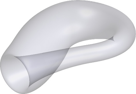
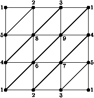
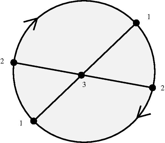
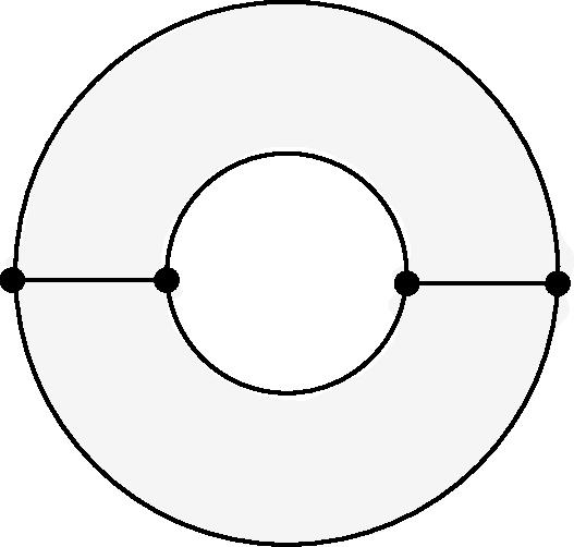
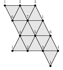
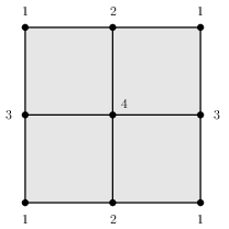
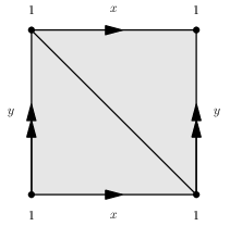
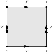
As just explained, the representations of spaces as simplicial complexes and regular CW complexes have their limitations. One limitation is that the number of cells needed to describe a space can be unnecessarily large. A minimal simplicial complex structure for the torus has 7 vertices, 21 edges and 14 triangles. A minimal regular CW-complex structure for the torus has 4 vertices, 8 edges and 4 cells of dimension 2. By using simplicial sets (which are like simplicial complexes except that they allow the freedom to attach simplicial cells by gluing their boundary non-homeomorphically) one obtains a minimal triangulation of the torus involving 1 vertex, 3 edges and 2 cells of dimension 2. By using non-regular CW-complexes one obtains a minimal cell structure involving 1 vertex, 2 edges and 1 cell of dimension 2. Minimal cell structures (in the four different categories) for the torus are illustrated as follows.
A second limitation to our representations of simplicial and regular CW-complexes is that they apply only to structures with finitely many cells. They do no apply, for instance, to the simplicial complex structure on the real line R in which each each integer n is a vertex and each interval [n,n+1] is an edge.
Simplicial sets provide one approach to the efficient combinatorial representation of certain spaces. So too do cubical sets (the analogues of simplicial sets in which each cell has the combinatorics of an n-cube rather than an n-simplex). Neither of these two approaches has been implemented in HAP.
Simplicial sets endowed with the action of a (possibly infinite) group G provide for an efficient representation of (possibly infinite) cell structures on a wider class of spaces. Such a structure can be made precise and is known as a simplicial group. Some functionality for simplicial groups is implemented in HAP and described in Chapter 12.
A regular CW-complex endowed with the action of a (possibly infinite) group G is an alternative approach to the efficient combinatorial representation of (possibly infinite) cell structures on spaces. Much of HAP is focused on this approach. As a first example of the idea, the following commands construct the infinite regular CW-complex Y=widetilde T arising as the universal cover of the torus T= S^1× S^1 where T is given the above minimal non-regular CW structure involving 1 vertex, 2 edges, and 1 cell of dimension 2. The homology H_n(T, Z) is computed and the fundamental group of the torus T is recovered.
gap> F:=FreeGroup(2);;x:=F.1;;y:=F.2;;
gap> G:=F/[ x*y*x^-1*y^-1 ];;
gap> Y:=EquivariantTwoComplex(G);
Equivariant CW-complex of dimension 2

gap> C:=ChainComplexOfQuotient(Y);
Chain complex of length 2 in characteristic 0 .

gap> Homology(C,0);
[ 0 ]
gap> Homology(C,1);
[ 0, 0 ]
gap> Homology(C,2);
[ 0 ]
gap> FundamentalGroupOfQuotient(Y);
<fp group of size infinity on the generators [ f1, f2 ]>
As a second example, the following comands load group number 9 in the library of 3-dimensional crystallographic groups. They verify that G acts freely on R^3 (i.e. G is a Bieberbach group) and then construct a G-equivariant CW-complex Y= R^3 corresponding to the tessellation of R^3 by a fundamental domain for G. Finally, the cohomology H_n(M, Z) of the 3-dimensional closed manifold M= R^3/G is computed. The manifold M is seen to be non-orientable (since it's top-dimensional homology is trivial) and has a non-regular CW structure with 1 vertex, 3 edges, 3 cells of dimension 2, and 1 cell of dimension 3. (This example uses Polymake software.)
gap> G:=SpaceGroup(3,9);;
gap> IsAlmostBieberbachGroup(Image(IsomorphismPcpGroup(G)));
true
gap> Y:=EquivariantEuclideanSpace(G,[0,0,0]);
Equivariant CW-complex of dimension 3

gap> Y!.dimension(0);
1
gap> Y!.dimension(1);
3
gap> Y!.dimension(2);
3
gap> Y!.dimension(3);
1
gap> C:=ChainComplexOfQuotient(Y);
Chain complex of length 3 in characteristic 0 .

gap> Homology(C,0);
[ 0 ]
gap> Homology(C,1);
[ 0, 0 ]
gap> Homology(C,2);
[ 2, 0 ]
gap> Homology(C,3);
[  ]
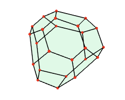
The fundamental domain for the action of G in the above example is constructed to be the Dirichlet-Voronoi region in R^3 whose points are closer to the origin v=(0,0,0) than to any other point v^g in the orbit of the origin under the action of G. This fundamental domain can be visualized as follows.
gap> F:=FundamentalDomainStandardSpaceGroup([0,0,0],G);
<polymake object>
gap> Polymake(F,"VISUAL");
Other fundamental domains for the same group action can be obtained by choosing some other starting vector v. For example:
gap> F:=FundamentalDomainStandardSpaceGroup([1/2,1/3,1/5],G);;
gap> Polymake(F,"VISUAL");

gap> F:=FundamentalDomainStandardSpaceGroup([1/7,1/2,1/2],G);
gap> Polymake(F,"VISUAL");
If a discrete group G acts on Euclidean space or hyperbolic space with finite stabilizer groups then we say that the quotient space obtained by killing the action of G an an orbifold. If the stabilizer groups are all trivial then the quotient is of course a manifold.
An orbifold is represented as a G-equivariant regular CW-complex together with the stabilizer group for a representative of each orbit of cells and its subgroup consisting of those group elements that preserve the cell orientation. HAP stores orbifolds using the data type of non-free resolution and uses them mainly as a first step in constructing free ZG-resolutions of Z.
The following commands use an 8-dimensional equivariant deformation retract of a GL_3( Z[ i])-orbifold structure on hyperbolic space to compute H_5(GL_3( Z[ i], Z) = Z_2^5⊕ Z_4^2. (The deformation retract is stored in a library and was supplied by Mathieu Dutour Sikiric.)
gap> Orbifold:=ContractibleGcomplex("PGL(3,Z[i])");
Non-free resolution in characteristic 0 for matrix group .
No contracting homotopy available.

gap> R:=FreeGResolution(Orbifold,6);
Resolution of length 5 in characteristic 0 for matrix group .
No contracting homotopy available.

gap> Homology(TensorWithIntegers(R),5);
[ 2, 2, 2, 2, 2, 4, 4 ]
The next example computes an orbifold structure on R^4, and then the first 12 degrees of a free resolution/classifying space, for the second 4-dimensional crystallographic group G in the library of crystallographic groups. The resolution is shown to be periodic of period 2 in degrees ≥ 5. The cohomology is seen to have 11 ring generators in degree 2 and no further ring generators. The cohomology groups are: $$H^n(G,\mathbb Z) =\left( \begin{array}{ll} 0, & {\rm odd~} n\ge 1\\ \mathbb Z_2^5 \oplus \mathbb Z^6, & n=2\\ \mathbb Z_2^{15}\oplus \mathbb Z, & n=4\\ \mathbb Z_2^{16}, & {\rm even~} n \ge 6 .\\ \end{array}\right.$$
gap> G:=SpaceGroup(4,2);;
gap> R:=ResolutionCubicalCrystGroup(G,12);
Resolution of length 12 in characteristic 0 for <matrix group with
5 generators> .

gap> R!.dimension(5);
16
gap> R!.dimension(7);
16
gap> List([1..16],k->R!.boundary(5,k)=R!.boundary(7,k));
[ true, true, true, true, true, true, true, true, true, true, true, true,
  true, true, true, true ]

gap> C:=HomToIntegers(R);
Cochain complex of length 12 in characteristic 0 .

gap> Cohomology(C,0);
[ 0 ]
gap> Cohomology(C,1);
[  ]
gap> Cohomology(C,2);
[ 2, 2, 2, 2, 2, 0, 0, 0, 0, 0, 0 ]
gap> Cohomology(C,3);
[  ]
gap> Cohomology(C,4);
[ 2, 2, 2, 2, 2, 2, 2, 2, 2, 2, 2, 2, 2, 2, 2, 0 ]
gap> Cohomology(C,5);
[  ]
gap> Cohomology(C,6);
[ 2, 2, 2, 2, 2, 2, 2, 2, 2, 2, 2, 2, 2, 2, 2, 2 ]
gap> Cohomology(C,7);
[  ]

gap> IntegralRingGenerators(R,1);
[  ]
gap> IntegralRingGenerators(R,2);
[ [ 1, 0, 0, 0, 0, 0, 0, 0, 0, 0, 0 ], [ 0, 1, 0, 0, 0, 0, 0, 0, 0, 0, 0 ],
  [ 0, 0, 1, 0, 0, 0, 0, 0, 0, 0, 0 ], [ 0, 0, 0, 1, 0, 0, 0, 0, 0, 0, 0 ],
  [ 0, 0, 0, 0, 1, 0, 0, 0, 0, 0, 0 ], [ 0, 0, 0, 0, 0, 1, 0, 0, 0, 0, 0 ],
  [ 0, 0, 0, 0, 0, 0, 1, 0, 0, 0, 0 ], [ 0, 0, 0, 0, 0, 0, 0, 1, 0, 0, 0 ],
  [ 0, 0, 0, 0, 0, 0, 0, 0, 1, 0, 0 ], [ 0, 0, 0, 0, 0, 0, 0, 0, 0, 1, 0 ],
  [ 0, 0, 0, 0, 0, 0, 0, 0, 0, 0, 1 ] ]
gap> IntegralRingGenerators(R,3);
[  ]
gap> IntegralRingGenerators(R,4);
[  ]
gap> IntegralRingGenerators(R,5);
[  ]
gap> IntegralRingGenerators(R,6);
[  ]
gap> IntegralRingGenerators(R,7);
[  ]
gap> IntegralRingGenerators(R,8);
[  ]
gap> IntegralRingGenerators(R,9);
[  ]
gap> IntegralRingGenerators(R,10);
[  ]
A group G with a finite index torsion free nilpotent subgroup admits a resolution which is periodic in sufficiently high degrees if and only if all of its finite index subgroups admit periodic resolutions. The following commands identify the 99 3-dimensional space groups (respectively, the 1191 4-dimensional space groups) that admit a resolution which is periodic in degrees > 3 (respectively, in degrees > 4).
gap> L3:=Filtered([1..219],k->IsPeriodicSpaceGroup(SpaceGroup(3,k)));
[ 1, 2, 3, 4, 5, 6, 7, 8, 9, 11, 12, 13, 15, 17, 18, 19, 21, 24, 26, 27, 28,
  29, 30, 31, 32, 33, 34, 36, 37, 39, 40, 41, 43, 45, 46, 52, 54, 55, 56, 58,
  61, 62, 74, 75, 76, 77, 78, 79, 80, 81, 84, 85, 87, 89, 92, 98, 101, 102,
  107, 111, 119, 140, 141, 142, 143, 144, 145, 146, 147, 148, 149, 150, 151,
  152, 153, 154, 155, 157, 159, 161, 162, 163, 164, 165, 166, 168, 171, 172,
  174, 175, 176, 178, 180, 186, 189, 192, 196, 198, 209 ]

gap> L4:=Filtered([1..4783],k->IsPeriodicSpaceGroup(SpaceGroup(4,k)));
[ 1, 2, 3, 4, 5, 6, 7, 8, 9, 11, 12, 13, 15, 16, 17, 18, 19, 20, 22, 23, 25,
  26, 29, 30, 31, 32, 33, 34, 35, 36, 37, 38, 39, 40, 42, 43, 44, 46, 47, 48,
  49, 50, 51, 52, 53, 54, 55, 56, 58, 59, 60, 61, 62, 63, 65, 66, 68, 69, 70,
  71, 73, 74, 75, 76, 77, 78, 79, 80, 81, 82, 83, 84, 85, 86, 87, 89, 90, 91,
  93, 94, 95, 96, 97, 98, 99, 101, 102, 103, 104, 105, 107, 108, 109, 110,
  111, 113, 115, 116, 118, 119, 120, 121, 122, 124, 126, 127, 128, 130, 131,
  134, 141, 144, 145, 149, 151, 153, 154, 155, 156, 157, 158, 159, 160, 162,
  163, 165, 167, 168, 169, 170, 171, 172, 173, 174, 176, 178, 179, 180, 187,
  188, 197, 198, 202, 204, 205, 206, 211, 212, 219, 220, 222, 226, 233, 237,
  238, 239, 240, 241, 242, 243, 244, 245, 247, 248, 249, 250, 251, 253, 254,
  255, 256, 257, 259, 260, 261, 263, 264, 265, 266, 267, 269, 270, 271, 273,
  275, 277, 278, 279, 281, 283, 285, 290, 292, 296, 297, 298, 299, 300, 301,
  303, 304, 305, 314, 316, 317, 319, 327, 328, 329, 333, 335, 342, 355, 357,
  358, 359, 361, 362, 363, 365, 366, 367, 368, 369, 370, 372, 374, 376, 378,
  381, 384, 385, 386, 387, 388, 389, 390, 391, 392, 393, 394, 395, 396, 397,
  398, 399, 400, 401, 402, 404, 405, 406, 407, 408, 409, 410, 411, 412, 413,
  414, 415, 416, 417, 418, 419, 421, 422, 423, 424, 425, 426, 427, 428, 429,
  430, 431, 432, 433, 434, 435, 436, 437, 438, 439, 440, 442, 443, 444, 445,
  446, 447, 448, 450, 451, 458, 459, 462, 464, 465, 466, 467, 469, 470, 473,
  477, 478, 479, 482, 483, 484, 485, 486, 493, 495, 497, 501, 502, 503, 504,
  505, 507, 508, 512, 514, 515, 516, 517, 522, 524, 525, 526, 527, 533, 537,
  539, 540, 541, 542, 543, 544, 546, 548, 553, 555, 558, 562, 564, 565, 566,
  567, 568, 571, 572, 573, 574, 576, 577, 580, 581, 582, 589, 590, 591, 593,
  596, 598, 599, 612, 613, 622, 623, 624, 626, 632, 641, 647, 649, 651, 652,
  654, 656, 657, 658, 659, 661, 662, 663, 665, 666, 667, 668, 669, 670, 671,
  672, 674, 676, 677, 678, 679, 680, 682, 683, 684, 686, 688, 689, 690, 691,
  692, 694, 696, 697, 698, 699, 700, 702, 708, 710, 712, 714, 716, 720, 722,
  728, 734, 738, 739, 741, 742, 744, 745, 752, 754, 756, 757, 758, 762, 763,
  769, 770, 778, 779, 784, 788, 790, 800, 801, 843, 845, 854, 855, 856, 857,
  865, 874, 900, 904, 909, 911, 913, 915, 916, 917, 919, 920, 921, 922, 923,
  924, 925, 926, 927, 929, 931, 932, 933, 934, 936, 938, 940, 941, 943, 945,
  946, 953, 955, 956, 958, 963, 966, 972, 973, 978, 979, 981, 982, 983, 985,
  987, 988, 989, 991, 992, 993, 995, 996, 998, 999, 1000, 1003, 1011, 1022,
  1024, 1025, 1026, 1162, 1167, 1236, 1237, 1238, 1239, 1240, 1241, 1242,
  1243, 1244, 1246, 1248, 1250, 1255, 1264, 1267, 1270, 1273, 1279, 1280,
  1281, 1283, 1284, 1289, 1291, 1293, 1294, 1324, 1325, 1326, 1327, 1328,
  1329, 1330, 1331, 1332, 1333, 1334, 1335, 1336, 1337, 1338, 1339, 1340,
  1341, 1343, 1345, 1347, 1348, 1349, 1350, 1351, 1352, 1354, 1356, 1357,
  1358, 1359, 1361, 1363, 1365, 1367, 1372, 1373, 1374, 1375, 1376, 1377,
  1378, 1379, 1380, 1381, 1382, 1383, 1384, 1385, 1386, 1387, 1388, 1389,
  1390, 1393, 1395, 1397, 1399, 1400, 1401, 1404, 1405, 1408, 1410, 1419,
  1420, 1421, 1422, 1424, 1425, 1426, 1428, 1429, 1438, 1440, 1441, 1442,
  1443, 1444, 1445, 1449, 1450, 1451, 1456, 1457, 1460, 1461, 1462, 1464,
  1465, 1470, 1472, 1473, 1477, 1480, 1481, 1487, 1488, 1489, 1493, 1494,
  1495, 1501, 1503, 1506, 1509, 1512, 1515, 1518, 1521, 1524, 1527, 1530,
  1532, 1533, 1534, 1537, 1538, 1541, 1542, 1544, 1547, 1550, 1552, 1553,
  1554, 1558, 1565, 1566, 1568, 1573, 1644, 1648, 1673, 1674, 1700, 1702,
  1705, 1713, 1714, 1735, 1738, 1740, 1741, 1742, 1743, 1744, 1745, 1746,
  1747, 1748, 1749, 1750, 1751, 1752, 1753, 1754, 1755, 1756, 1757, 1759,
  1761, 1762, 1763, 1765, 1767, 1768, 1769, 1770, 1771, 1772, 1773, 1774,
  1775, 1778, 1779, 1782, 1783, 1785, 1787, 1788, 1789, 1791, 1793, 1795,
  1797, 1798, 1799, 1800, 1801, 1803, 1806, 1807, 1809, 1810, 1811, 1813,
  1815, 1821, 1822, 1823, 1828, 1829, 1833, 1837, 1839, 1842, 1845, 1848,
  1850, 1851, 1852, 1854, 1856, 1857, 1858, 1859, 1860, 1861, 1863, 1866,
  1870, 1873, 1874, 1877, 1880, 1883, 1885, 1886, 1887, 1889, 1892, 1895,
  1915, 1918, 1920, 1923, 1925, 1927, 1928, 1930, 1952, 1953, 1954, 1955,
  2045, 2047, 2049, 2051, 2053, 2054, 2055, 2056, 2057, 2059, 2067, 2068,
  2072, 2075, 2076, 2079, 2084, 2087, 2088, 2092, 2133, 2135, 2136, 2137,
  2139, 2140, 2170, 2171, 2196, 2224, 2234, 2236, 2238, 2254, 2355, 2356,
  2386, 2387, 2442, 2445, 2448, 2451, 2478, 2484, 2487, 2490, 2493, 2496,
  2499, 2502, 2508, 2511, 2514, 2517, 2520, 2523, 2550, 2553, 2559, 2621,
  2624, 2648, 2650, 3046, 3047, 3048, 3049, 3050, 3051, 3052, 3053, 3054,
  3055, 3056, 3057, 3058, 3059, 3060, 3061, 3062, 3063, 3064, 3065, 3066,
  3067, 3068, 3069, 3070, 3071, 3072, 3073, 3074, 3075, 3076, 3077, 3078,
  3079, 3080, 3081, 3082, 3083, 3084, 3085, 3086, 3087, 3089, 3090, 3091,
  3094, 3095, 3096, 3099, 3100, 3101, 3104, 3105, 3106, 3109, 3110, 3111,
  3112, 3113, 3114, 3115, 3117, 3119, 3120, 3121, 3122, 3123, 3124, 3125,
  3127, 3128, 3129, 3130, 3131, 3132, 3133, 3135, 3137, 3139, 3141, 3142,
  3143, 3144, 3145, 3149, 3151, 3152, 3153, 3154, 3155, 3157, 3159, 3160,
  3161, 3162, 3163, 3169, 3170, 3171, 3172, 3173, 3174, 3175, 3177, 3179,
  3180, 3181, 3182, 3183, 3184, 3185, 3187, 3188, 3189, 3190, 3191, 3192,
  3193, 3195, 3197, 3199, 3200, 3201, 3204, 3206, 3207, 3208, 3209, 3210,
  3212, 3214, 3215, 3216, 3217, 3218, 3226, 3234, 3235, 3236, 3244, 3252,
  3253, 3254, 3260, 3268, 3269, 3270, 3278, 3280, 3281, 3282, 3283, 3284,
  3285, 3286, 3287, 3288, 3289, 3290, 3291, 3292, 3295, 3296, 3298, 3299,
  3302, 3303, 3306, 3308, 3309, 3310, 3311, 3312, 3313, 3314, 3315, 3316,
  3317, 3318, 3319, 3320, 3322, 3324, 3326, 3327, 3329, 3330, 3338, 3345,
  3346, 3347, 3348, 3350, 3351, 3352, 3354, 3355, 3356, 3359, 3360, 3361,
  3362, 3374, 3375, 3383, 3385, 3398, 3399, 3417, 3418, 3419, 3420, 3422,
  3424, 3426, 3428, 3446, 3447, 3455, 3457, 3469, 3471, 3521, 3523, 3524,
  3525, 3530, 3531, 3534, 3539, 3542, 3545, 3548, 3550, 3551, 3554, 3557,
  3579, 3580, 3830, 3831, 3832, 3833, 3835, 3837, 3839, 3849, 3851, 3877,
  3938, 3939, 3949, 3951, 3952, 3958, 3960, 3962, 3963, 3964, 3966, 3968,
  3972, 3973, 3975, 4006, 4029, 4030, 4033, 4034, 4037, 4038, 4046, 4048,
  4050, 4062, 4064, 4067, 4078, 4081, 4089, 4090, 4114, 4138, 4139, 4140,
  4141, 4146, 4147, 4148, 4149, 4154, 4155, 4169, 4171, 4175, 4180, 4183,
  4188, 4190, 4204, 4205, 4223, 4224, 4225, 4254, 4286, 4289, 4391, 4397,
  4496, 4499, 4500, 4501, 4502, 4504, 4508, 4510, 4521, 4525, 4544, 4559,
  4560, 4561, 4562, 4579, 4580, 4581, 4583, 4587, 4597, 4598, 4599, 4600,
  4651, 4759, 4760, 4761, 4762, 4766 ]
generated by GAPDoc2HTML